We have late open sourced Cleora — an ultra fast vertex embedding tool for graphs & hypergraphs. Cleora can ingest any categorical, relational data and turn it into vector embeddings of entities. It is extremely fast, while offering very competitive quality of results. In fact, for reasons outlined below, it may be the fastest hypergraph embedding tool possible in practice.
Now, we print the Cleora whitepaper on arXiv for all to read. The whitepaper offers a peek into the interior workings of the algorithm, as well as any interesting benchmarks.
We’ve been utilizing Cleora in production at Synerise for a fewer years now, handling terabytes of data for our customers. It has evolved from a script version written in Python & Numpy, went through a concurrent Scala implementation on the JVM, and now has reached maturity with a highly optimized version written in Rust.
Is there a hypergraph in your data? (Yes)
Not many people realize that hypergraphs are ubiquitous. If you have at least 1 relational table with 2 categorical columns, you indeed have a graph and 2 hypergraphs!
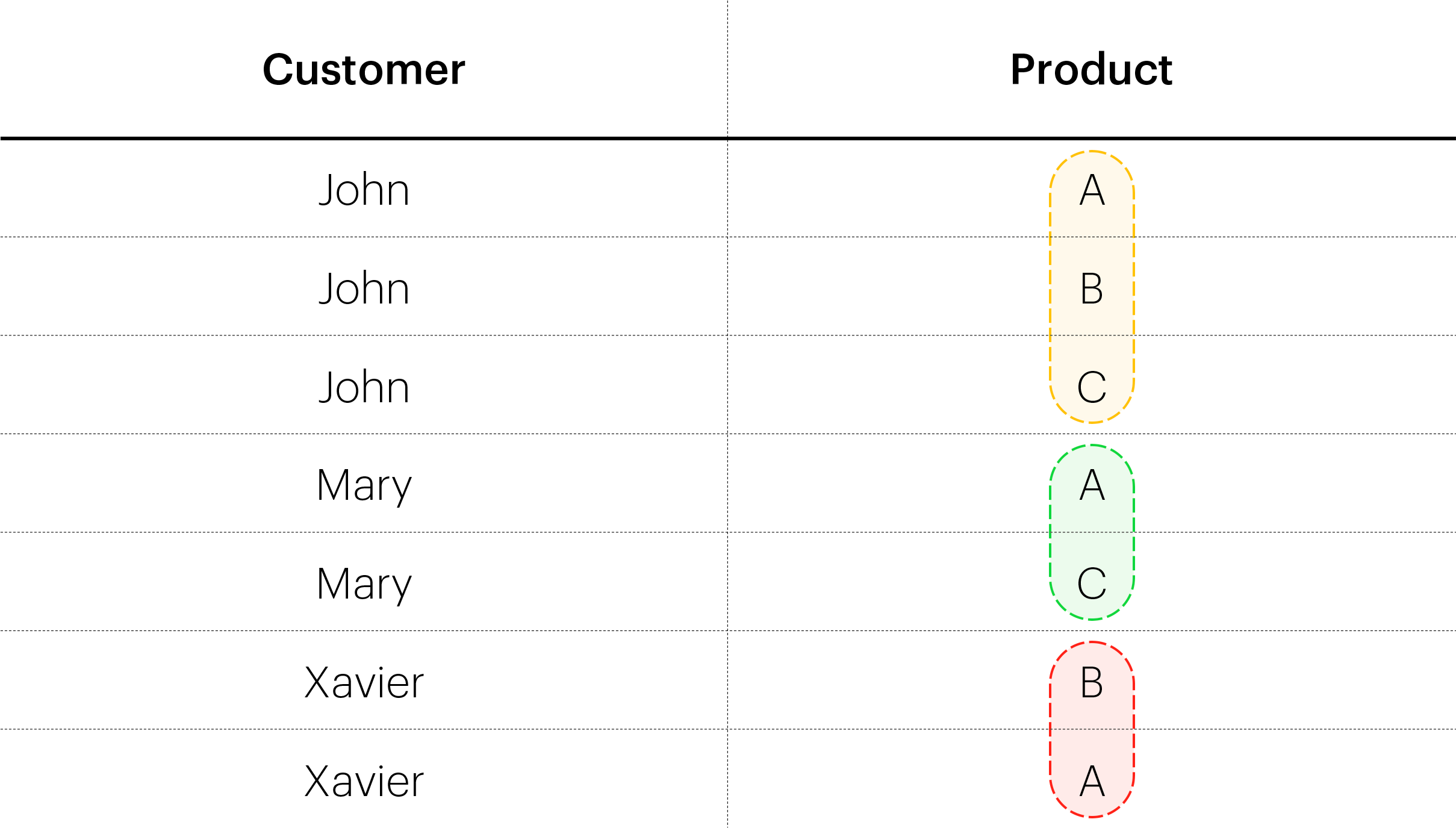
Let’s take a very simple example of a relational table:
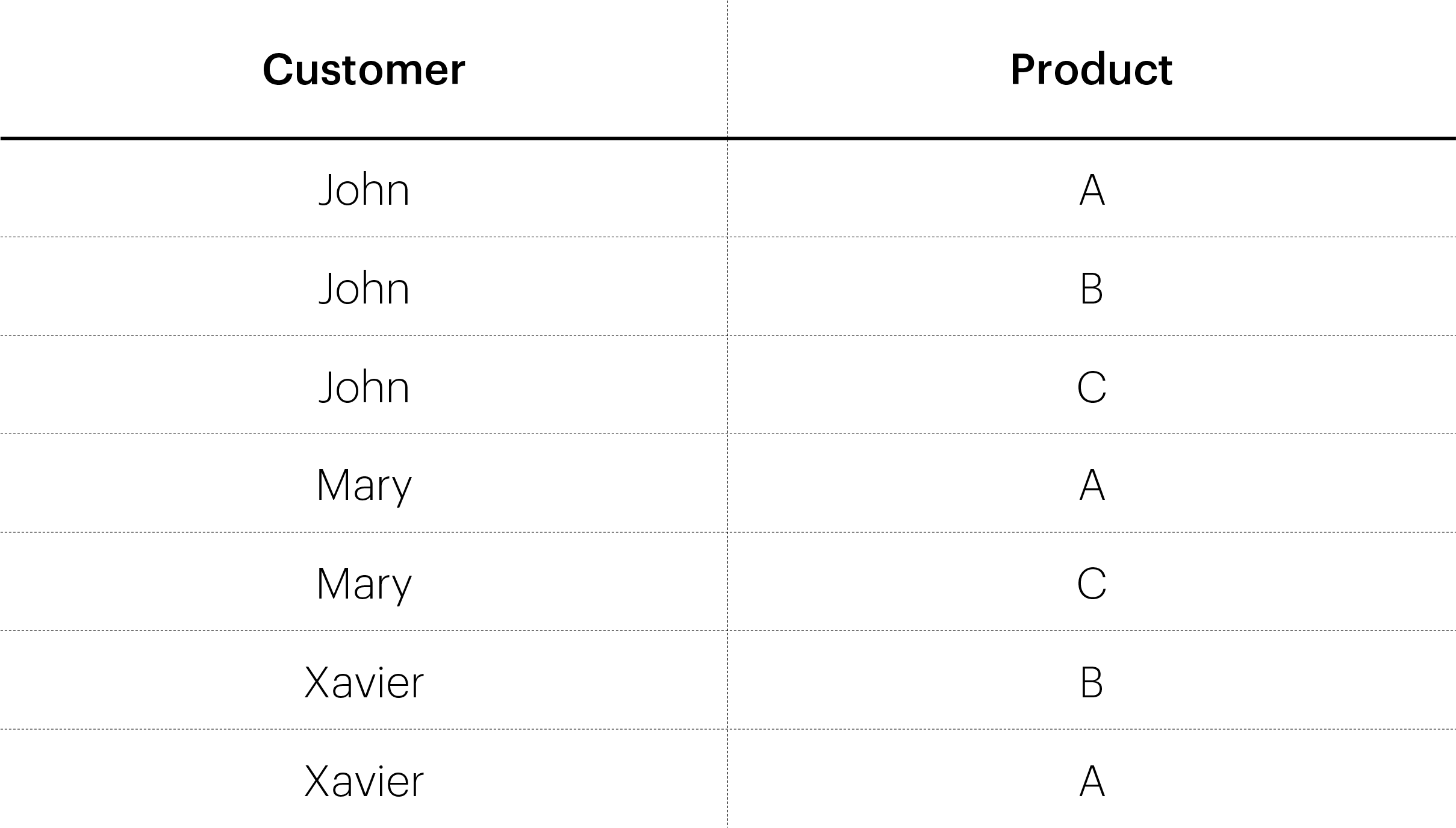 Example of a simple relational table.
It can be represented as a graph, with vertices (John, Mary, Xavier, A, B, C) as follows:
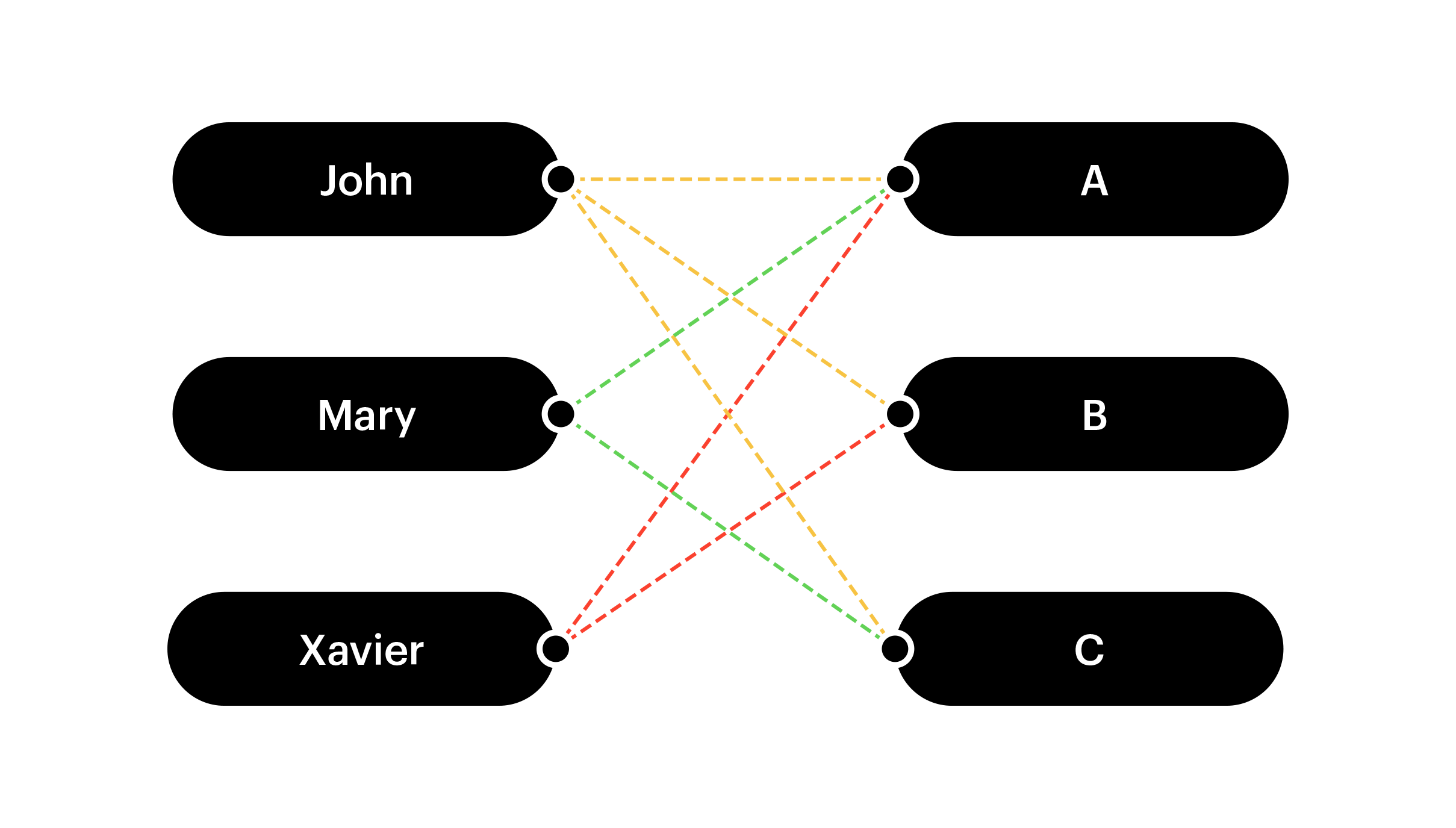
The edges of the graph correspond 1–1 to the rows in the table, e.g. (John , A), (Mary , C).
But there are hypergraphs lurking in this graph! Let’s treat Customers as generalized edges instead, and see what happens:
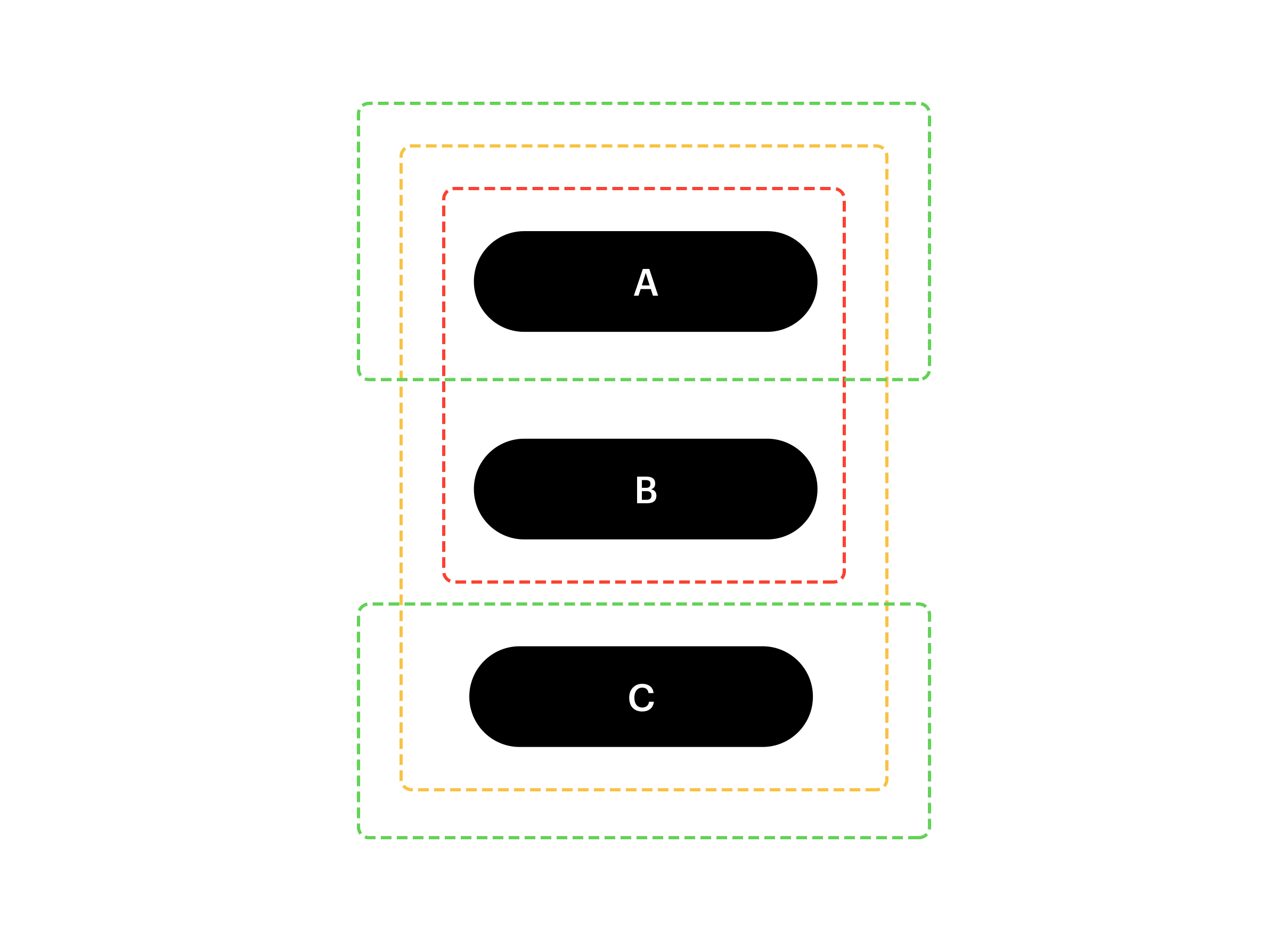
What we did here is — we’ve taken Products (A, B, C) as vertices, and treated Customers (John, Mary, Xavier) as hyperedges. We can think of this as a simple “group by” operation, where we group the Products by the Customers. It may be easier to visualize the hyperedges in the actual table:
So we have 3 hyperedges: (A, B, C), (A, C), and (B, A). announcement the first hyperedge has cardinality 3 — it spans 3 different vertices. That’s the hyperpart in a hypergraph — edges can span more than 2 vertices. We could have done the grouping the another way around (group Customers by Products), which would consequence in yet another hypergraph.
Why are hypergraphs more useful than graphs?
The graph format is highly limited, allowing only for links between 2 entities. On the another hand, hypergraphs let us to represent bigger relations.
For instance datasets of shopping baskets or user’s online sessions form natural hypergraphs. All the products in a buying basket are together bound by the relation of belonging to a single basket. All the items viewed during an online session, are powerfully coupled as well. And the number of items in both can be importantly larger than 2. Hence, a single basket is simply a hyperedge.
We have empirically confirmed that the hypergraph approach works much better than graphs for product embeddings, website embeddings & another akin data. It’s more expressive and captures the underlying data generating process better.
The good thing about Cleora is that it can handle both simple graphs and hypergraphs seamlessly, to produce entity embeddings!
What’s so peculiar about Cleora?
In addition to native support for hypergraphs, a fewer things make Cleora stand out from the crowd of vertex-embedding models:
- It has no training objective, in fact there is no optimization at all (which makes both determinism & utmost velocity possible)
- It’s deterministic — training from scratch on the same dataset will give the same results (there’s no request to re-align embeddings from multiple runs)
- It’s stable — if the data gets extended / modified a little, the output embeddings will only change a small (very useful erstwhile combined with e. g. unchangeable clustering)
- It supports approximate incremental embeddings for vertices unseen during training (solving the cold-start problem & limiting request for re-training)
- It’s highly scalable and inexpensive to use — we’ve embedded hypergraphs with 100s of billions of edges on a single device without GPUs
- It’s more than ~100x faster than any erstwhile approaches like DeepWalk. It likely is the fastest possible approach possible.
All of the above properties are either missing or impossible to achieve when utilizing another methods.
How is specified efficiency even possible?
There are 2 major kinds of vertex embedding methods. We unify & simplify both.
One large class of vertex embedding methods is based on random walks. These approaches take the input graph, and stochastically make “paths” (sequences of vertices) from a random walk on the graph. As if a bug was hopping from 1 vertex to another, along the edges. They are trained with stochastic gradient descent applied to various objectives, most of them akin to skip-gram or CBOW known from word2vec and can disagree somewhat in how the random walks are defined.
The another large class is based on Graph Convolutional Networks. These models treat the graph as an adjacency matrix, specify a “neighborhood mixing” operator called a graph convolution and any non-linearities in between. They can be trained with SGD applied to various objectives as well.
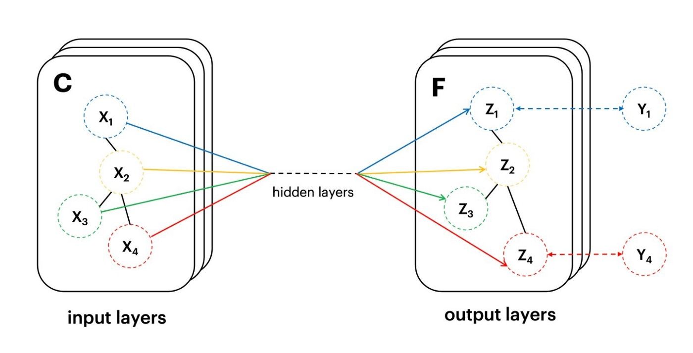
Cleora combines both intuitions into a simple solution. alternatively of sampling individual random walks from a graph, it represents the graph with its random walk as a Markov transition matrix. Multiplication of vertex embeddings by this matrix allows us to execute all the possible random walks in parallel, in a full deterministic way — with 1 large step.
During our work with Graph Convolutional Networks, we have noticed that contrary to our intuition, the effect imposed by non-linearities & dense layers in between convolutions is not expanding expressive power, but alternatively normalizing and stabilizing the embeddings. Graph convolutions execute a neighborhood smoothing operation, and for our purposes, everything else is redundant.
Once we strip all learnable parameters from a Graph Convolutional Network, all that remains is iterative matrix multiplication. Smoothing alone can be performed precisely by iterative multiplication with a Markov Transition Matrix. The problem with specified stochastic matrices is that for all non-trivial cases, their determinant is little than 1. This implies all the eigenvalues to be smaller than 1 as well — and under iterative multiplication would origin the norms of embedding vectors to vanish exponentially quickly.
To solve the vanishing norm problem, we re-normalize our embeddings after all iteration, projecting them onto a unit sphere.
This way we accomplish Cleora’s signature spherical embeddings, with random initialization, simple (sparse) matrix multiplication, zero learning and zero optimization. You truly can’t get much faster than this, without intentionally discarding any input data.
Given T — the embedding vectors, and M — the Markov transition matrix, we have:
That’s it. All it does is iterative vicinity smoothing & re-normalization. And seemingly that’s adequate for advanced quality vertex embeddings.
What about determinism and stability? Nobody else has that!
A common problem with vector embeddings is that:
- the embedding vectors change (rotation + noise) with all run on the same data
- the embedding vectors change (more drastically) erstwhile the data changes
All another methods execute any kind of stochastic optimization, and have any randomly-initialized parameters to be learned. Cleora doesn’t have any stochasticity whatsoever.
Given the perfect determinism and deficiency of learnable parameters of the algorithm itself, it suffices to initialize the embedding vectors in a deterministic way. Deterministic embedding vector initialization can be achieved utilizing independent pseudo-random hash functions (we chose xxhash). Mapping a vertex description to an integer hashcode, and mapping the integer to a floating point number in the scope of (-1, 1), gives a Uniform(-1, 1) distribution utilized in the paper. 1 can repeat with N different seeds, to get a vector of dimension N.
In principle, 1 could besides easy execute Gaussian (and other) initialization this way, plugging in the U(-1,1) samples into the desired inverse cumulative distribution function. utilizing another distributions did not aid Cleora, but it’s a good hack to be aware of.
So, why is it written in Rust?
Versions written in Python + Numpy had problems with very slow sparse matrix multiplication. A version written in Scala has served us nicely for a fewer months, but had problems with excessive memory consumption for very large graphs.
The final Rust implementation is hyper-optimized for:
- extremely fast matrix multiplication
- minimal memory overhead
It works just as it should.
What’s next?
We’re utilizing Cleora in our products, but we have besides successfully applied Cleora (as 1 component of a larger stack) in ML competitions, specified as the fresh Booking.com Data Challenge, where we took 2nd place, narrowly beaten by the Nvidia team.
The goal of Booking Data Challenge was stated as:
Use a dataset based on millions of real anonymized accommodation reservations to come up with a strategy for making the best advice for their next destination in real-time.
A short while back, we have besides applied Cleora & taken 1st place at Rakuten Data Challenge 2020 in the category of Cross-Modal Retrieval.
The goal of Rakuten Data Challenge was stated as:
Given an held-out test set of product items with their titles and (possibly empty) descriptions, foretell the best image from among a set of test images that correspond to the products in the test set
We usually combine Cleora with a more advanced method from our AI squad called EMDE — An Efficient Manifold Density Estimator for advanced dimensional spaces.
We feel Cleora is simply a tool worth sharing. So check out the paper, take a look into our github repo and calculate any embeddings!
And if you’re in the temper to contribute to an open-source project, Cleora could be extended with deterministic initialization from vertex attributes / feature vectors (e.g. via deterministic random projections).