EMDE – motivations, explanations and intuitions
In this article we supply any intuitive explanations of our objectives and theoretical background of the Efficient Manifold Density Estimator (EMDE). We describe our inspirations and thought process which led to the formulation of the algorithm. Then, we dive further into technicalities to show how the intuitions link to actual mathematical formulas behind the algorithm.
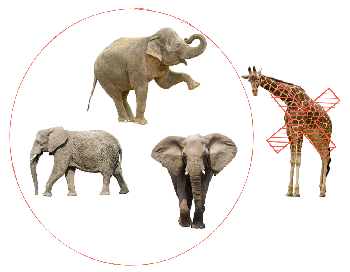
Research on the EMDE algorithm started from spotting respective shortcomings of current device learning methods. Let us consider an highly basic cognitive ability to group akin objects regardless of their individual differences. Even young children can group different pictures of elephants together and admit that a giraffe doesn’t belong to this group. These kinds of abilities are shown even in the behaviour of 10-month-old infants. It is not only a very basic skill but besides a very crucial 1 for another more complex processes. It allows to organize perception and cognition in a changing environment. By analogy to human cognition, we wanted to make an algorithm that would be able to solve this task in a simple way without a disproportionate computational overhead, i.e., with a single linear pass, without quadratic computational complexity.
Looking at this from a somewhat different angle: we wanted to aggregate various sets of vectors in a compressed representation, that can model membership function – recreate groupings created by object/event features represented by vectors. We were inspired by 2 algorithms: Count-Min Sketch (CMS) and Locality delicate Hashing. CMS is simply a very efficient algorithm utilized to approximate the number of occurrences of a given item in a data stream. The item number is incremented in multiple rows of a two-dimensional array (the sketch), where each row corresponds to a different hashing function. Then the minimum value for a given item across all hashing functions is an item number approximation. utilizing multiple hashing functions minimizes hash collisions impact. While CMS applies random hashes to item labels, LSH aims to put in the same bucket items that are close together in the input space. EMDE borrowed the thought of histogram-like number over many hashing functions from CMS and from LSH a space hashing approach that is aware of the input space geometry.
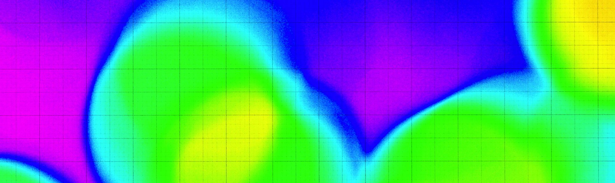
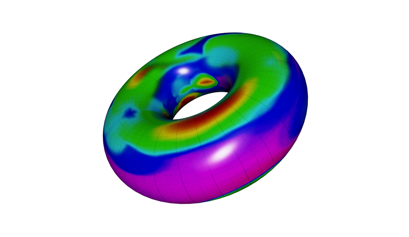
To realize the notion of input space geometry we request to introduce the concept of a data manifold. Formally speaking, a Riemannian manifold is simply a metric space that locally resembles Euclidean space close each point. The acquainted Euclidean space itself is in fact a basic example of a manifold. erstwhile we consider vectors representing any aspect of objects we want to aggregate, for example image embeddings, all our data points represented by these embeddings can be seen as points on a manifold. The closeness of 2 points on a manifold will represent the similarity of objects in real-life with respect to the features expressed by vectors spanning the manifold. To aggregate any subset of data points, e.g. acquisition past of a given user, we can represent it with a heatmap created over the manifold.
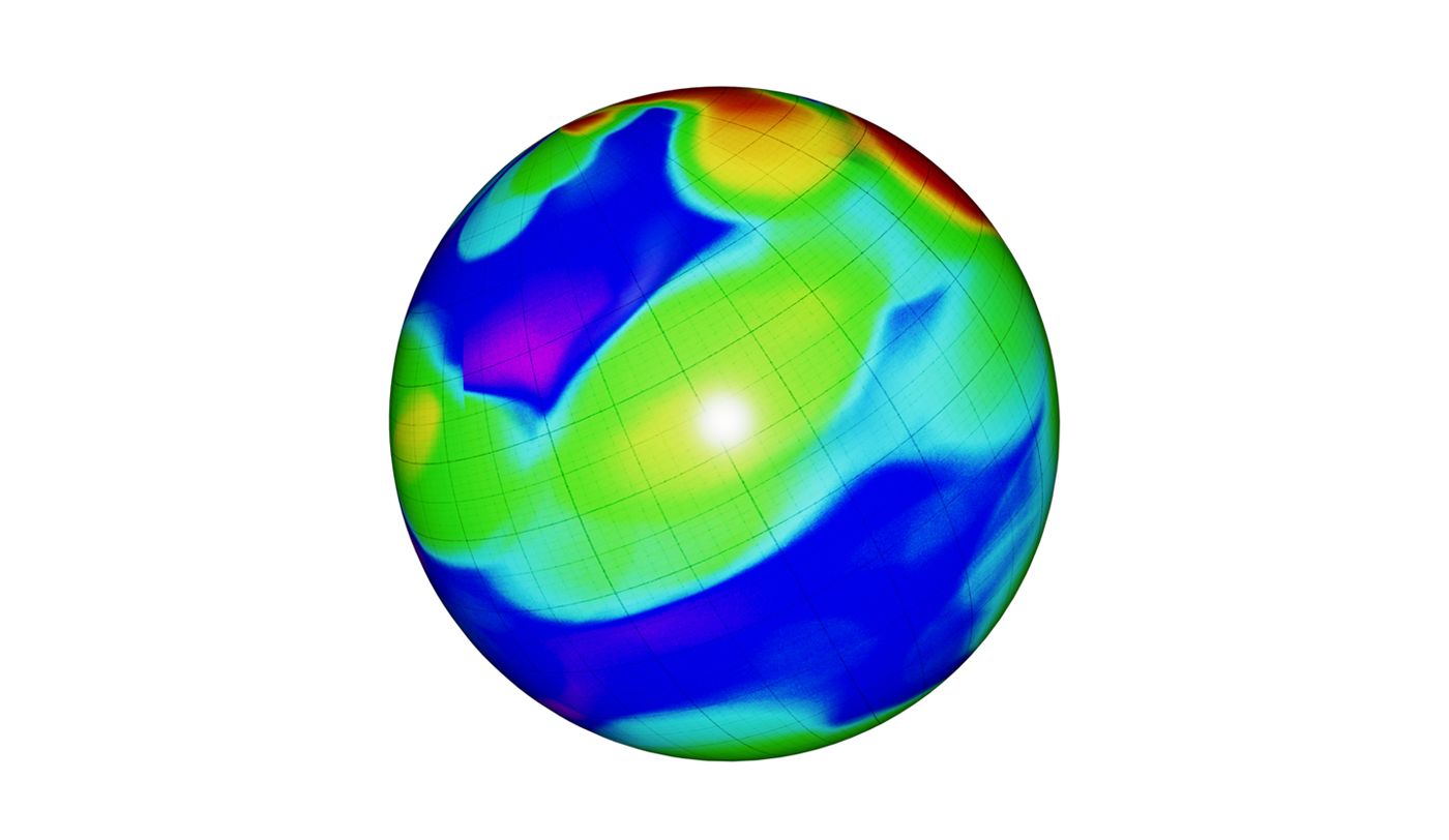
To make any intuitive knowing behind this idea, let’s consider a manifold example that we can easy put our finger on – the Earth’s surface. Imagine a script in which we want to present information about places that a individual visits and how frequently they visit these places. We could take a sphere representing the surface of the Earth and mark visited places with a heatmap. The lighter regions will represent places that are visited more often, and the darker regions places seldom visited or not visited at all.
Similar to the Earth surface, we can consider a manifold that is spanned by our image embeddings. It is crucial to note that the manifold is embedded in Rn, but is not the full Rn space. Image embeddings for all possible “images in the wild” will carve out a tiny fragment of Rn, and that fragment is our manifold of interest. We can, for example, make a heatmap where vectors representing products bought by a given user can be interpreted as “visited places” on a manifold. This heatmap will then inform us what kind of products (as described by their visual features) the user preferred in the past. If I bought many pairs of shoes and didn’t buy any swimwear, the region where shoe images reside will be brighter and the swimwear region will be completely dark. This way we can make accurate maps of user preferences.
However, we don’t request to limit ourselves to image embeddings, we can consider any kind of vector representation as textual embeddings of product descriptions or user-product interaction vectors. By combining these sources of information, we can make truly accurate models of user behavior. What is more, aggregating input in the form of heatmaps enables us to represent probability distributions, which is impossible erstwhile we usage pointwise averages, or sequential inputs. So, the question of how to pass these maps over manifolds to a device learning algorithm becomes crucial in our research. Also, erstwhile we consider a model output, we can represent it as a heatmap, for example expressing the probability of the next bought item. advice task can be then stated as uncovering the right mapping between these 2 heatmaps – the user behavioral model and the probability of a next bought item. The question remains how to transfer information from the manifold to the finite-size data structure.
From manifold to sketch
The closeness of 2 points on the manifold informs us that 2 objects are akin with respect to features encoded in vector representations spanning the manifold. Taking this fact into consideration we could divide manifold into regions and treat the vectors falling into the same region as representations of objects of 1 kind. Then we would simply add up vectors in each region to transform information from a manifold into a numerical structure.
Going back to the heatmap of visited places– how can we transform it into a numerical matrix? We can make usage of the fact that our globe is already divided into regions. For instance, we may number how many times a individual was in a given country. But what if we have data from 1 period and want to observe someone’s day to day patterns? We can then go to the lower levels, like regions, cities, districts, etc. However, the finer division we presume the higher the number of regions is and thus we end up with a very large and hard-to-process structure.
Similarly, we request to divide the manifold into regions, which will let us to make an accurate representation of an aggregated data heatmap. At the same time, the representation needs to be compact and easy to usage as a part of a device learning pipeline.
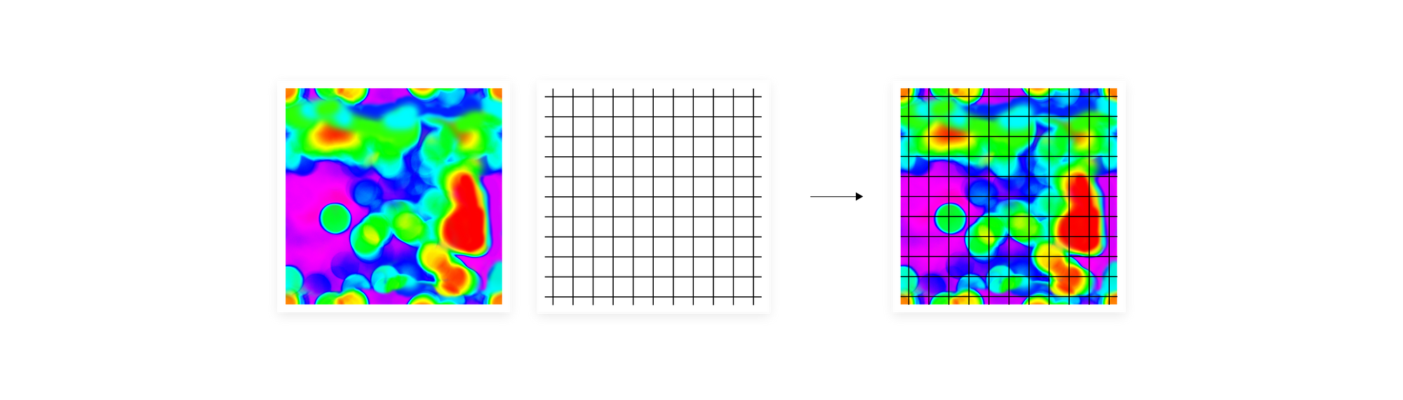
One solution will be to make an even grid over the heatmap and add up the vectors from each region. However, if we made the grid besides coarse, we would lose any pieces of information we wanted to transfer from the manifold. Also, this kind of division will consequence in alternatively noisy categories, where objects of different kinds will frequently fall into the same region. On the another hand, by making a grid besides fine-grained we end up with a immense matrix, highly hard to process. It may besides deficiency generalization, which was the point of aggregating vectors based on their closeness in the input space geometry, alternatively of passing them to the algorithm sequentially.
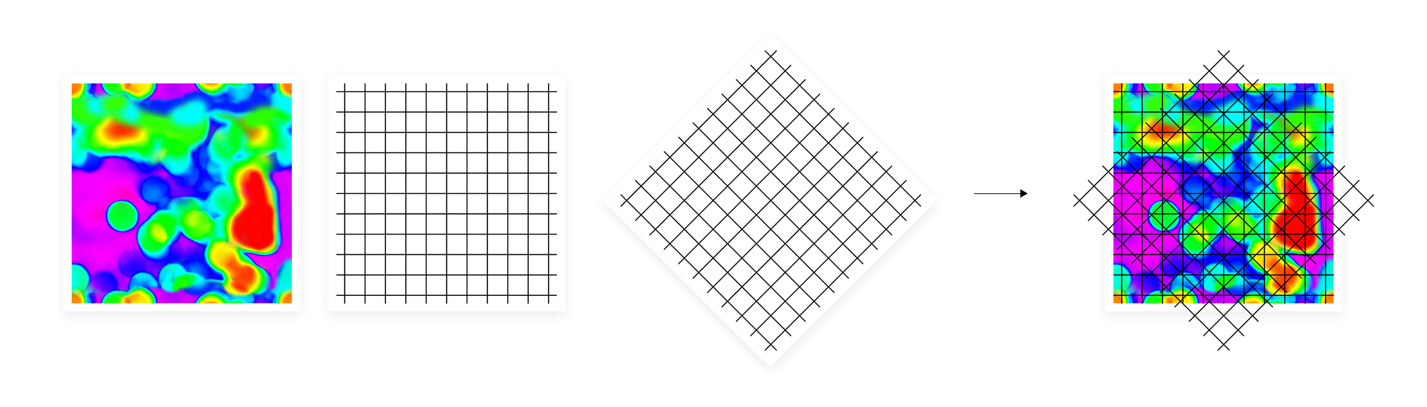
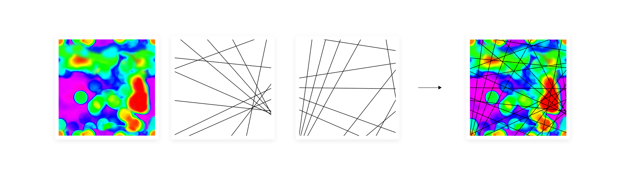
To overcome these obstacles, we make multiple independent manifold divisions. erstwhile we make 2 different grids and stack 1 on top of another, performing a geometric intersection, the number of regions that were created on the intersection of these 2 grids is much bigger than if we simply add up the number of regions from both grids. The larger the dimensionality of the first input space, the more subregions an intersection can give, with the advanced bound being exponential with respect to the number of different divisions. Usually, embeddings utilized in device learning as an input data representation are high-dimensional vectors so with the right number of separate manifold divisions, we can get a very high-resolution representation of a manifold. In a sense, we translate the heatmap drawn over the manifold into this kind of histogram on steroids. At the same time, we keep the final representation, a sketch, alternatively compact. Its width is defined by the number of regions in a single manifold division and depth is the number of separate divisions. The example size of a sketch utilized in our experiments is width 128 and depth 100.
However, dividing the manifold with an even grid can consequence in many empty regions or all data points falling into 1 region. To prevent this, we usage the quantile function erstwhile creating the hyperplanes dividing the manifold. This way we make certain that we divide manifold into non-empty regions in a density-dependent way.
Thus far we have provided any intuitive explanations of EMDE’s background. In the next section, we will present a step-by-step explanation of the algorithm itself and show how it can be utilized for model training and inference.
EMDE Step-by-step
Input data: vectors representing a given aspect of items we want to aggregate, e.g. embedding vectors of product descriptions, or Cleora embeddings (github repository) from behavioral user data
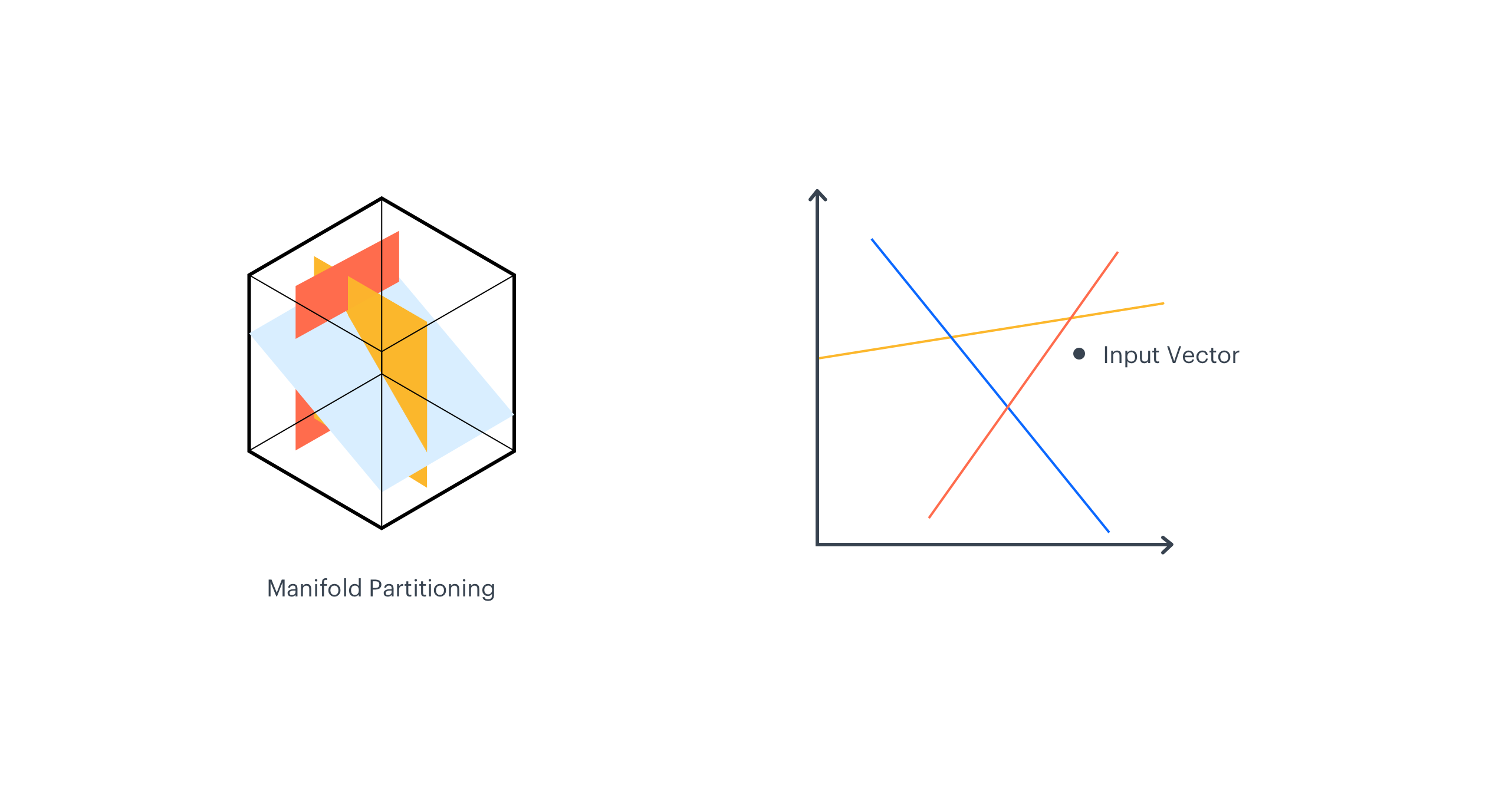
Manifold Partitioning
The central part of the EMDE algorithm is the data manifold partitioning procedure. First, K hyperplanes are selected to cut the manifold into 2K regions, and each region corresponds to 1 bucket in the final sketch. This makes the sketch_width dimension.
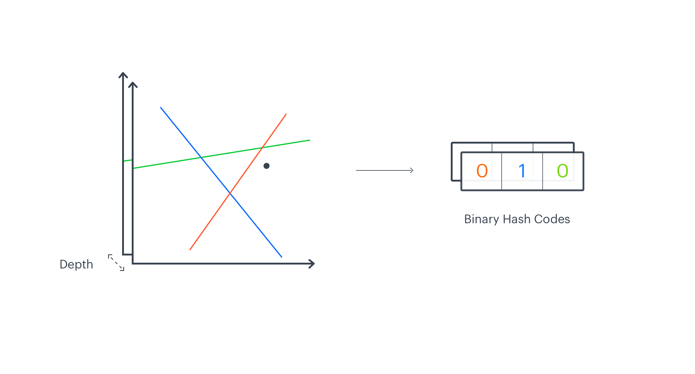
As each hyperplane divides manifold into 2 parts, we have K binary hash codes for a single input vector, which taken together represent the region that the vector falls into.
Hyperplane Selection
To avoid unutilized regions we want to cut the manifold into nonempty parts. To do so, we introduce the modified version of the LSH algorithm – Density-depended LSH. We make K random vectors ri and calculate hash codes with the provided formula:
hashi(v) = sgn(v · ri −bi)
where v represents the input vector and bi is simply a bias drawn from the data-dependent quantile function of v · ri
Adding Depth
In the erstwhile paragraph, we described how to make a single manifold division. In order to get a high-resolution representation, we request to make multiple independent divisions of a manifold. They will make the sketch_depth parameter. 1 independent partition creates 2K regions and each vector on a manifold falls into 1 of these regions. Next, we repeat manifold partitioning procedure, which results in creating different 2K regions. In this case, we end up with 2 binary vectors of a dimension K, each representing a region that a vector falls into in a given manifold division. We stack them together across the sketch_depth axis. Normally, the number of independent manifold divisions is higher. We can then presume that 2 akin vectors will frequently fall into the same region in different partitions.
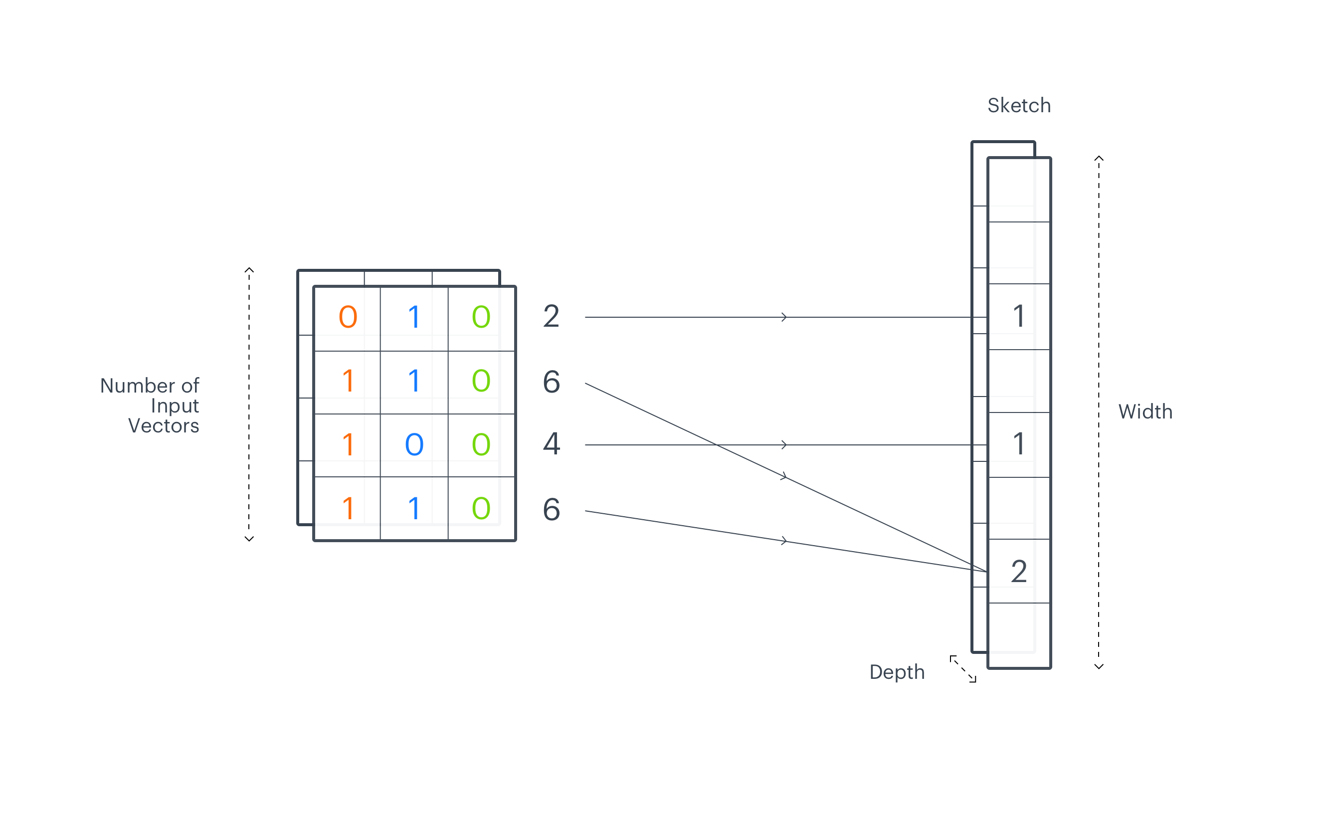
Sketches
The output of the EMDE algorithm is simply a sketch, an aggregated representation where each bucket stores the number of input vectors that fall into a peculiar region. Binary vectors calculated for all input embeddings are packed into integers we call codes. Codes represent the regions from the manifold division and indicate on which index of the final sketch to increment the count. This way we end up with an aggregated representation of input data. The described procedure is repeated separately on each depth-level. The final representation has 2 dimensions sketch_width – the number of regions from single manifold division (with K hyperplanes) and sketch_depth – the number of independent manifold divisions into sketch_width regions. To make a more robust representation we can concatenate sketches from different modalities like text, image, graphs.
Using EMDE for Recommendations
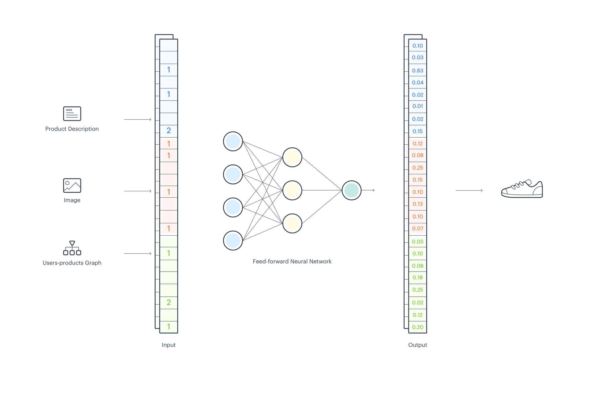
From the erstwhile part we know how to usage EMDE to make aggregated data representation, now let’s consider how to train a recommender strategy utilizing EMDE sketches. Based on user acquisition past we want to foretell the next items the user will buy. To make sketches, we usage product descriptions, pictures, and user-product interaction graph. We can usage 1 of the popular embedding methods for text and images. To make node embeddings, we usage our own model Cleora, but any another graph embedding method can be besides utilized with EMDE. For each input type, we make sketches separately and concatenate them.
To train a model we take acquisition histories of many users. For each user, we aggregate events before a time divided to make an input sketch and after the time divided to make the mark sketch – the purchases we want to predict. Data prepared this way are utilized to train a simple feed-forward neural network. The goal of training is to find the right mapping between the manifold regions that represents user past behavior/preferences to the manifold regions that represent the most probable next choices.
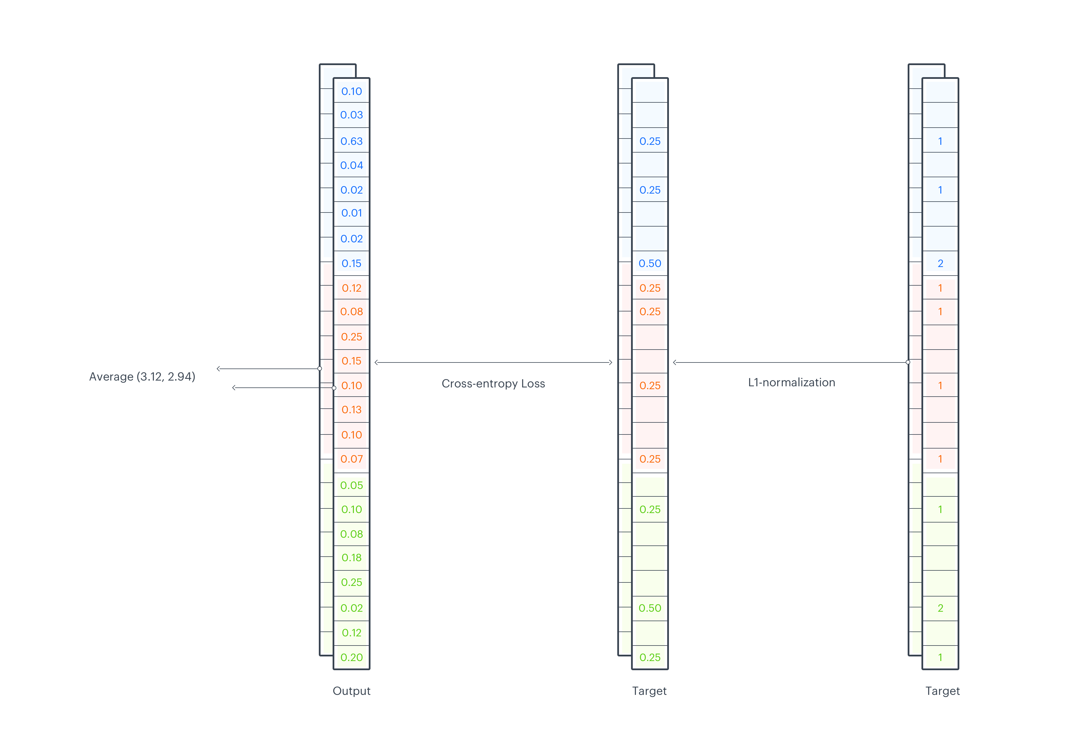
Loss function
To calculate the loss, first we request to L1-normalize the mark sketch, which then can be considered as a probability mass function of a discrete distribution. Next, we apply the softmax function on output logits and calculate cross entropy failure between an output and the target. All operations are done across sketch_width, so we end up with a separate failure value for each sketch_depth dimension. In the last step, we average them across depth.
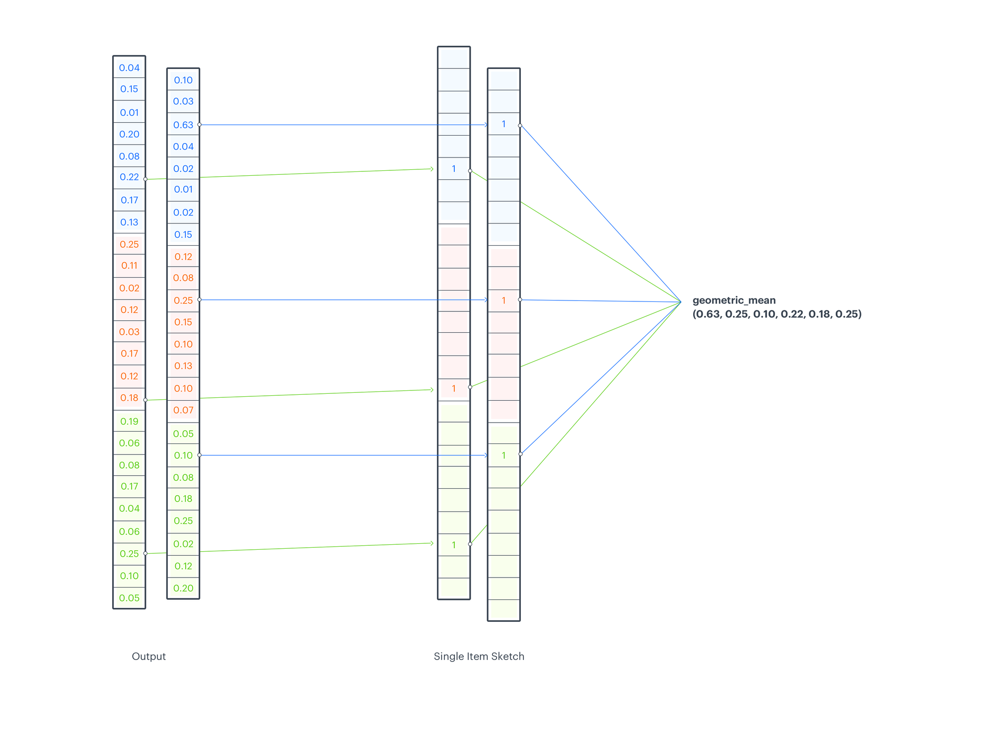
Prediction
To calculate a score for a advice candidate we look up scores from applicable indices of model output. For each depth-level and input kind we consider advice candidate code (representing the manifold region, that the candidate falls into) and we take the score from the output sketch, which was returned for a given code (sketch index). We aggregate them utilizing a geometric mean. The aggregation function differs from the 1 utilized in CMS (minimum operation), but while CMS operates on counts, EMDE at this point operates on probabilities.
This way we can make very powerful aggregated data “histograms” encoded in sketches and usage them to train a simple neural network. The aim of the model training is to map the regions of an input manifold to the regions of an output manifold. Map user preferences to the probability of the next bought object. What is worth noticing, with only 1 linear layer and no additional non-linearity, we are able to execute a very non-linear mapping between manifolds. This brings a shift in a current paradigm, where quite a few improvements – various initialization methods or residual connections, which are meant to facilitate NN training, make the overall strategy closer to a linear transformation.
To validate our approach and get the thought about the EMDE performance in comparison with another methods we took part in respective competitions: KDD Cup 2021, Twitter RecSys Challenge 2021, WSDM Booking.com Challenge 2021, SIGIR Rakuten Challenge 2020. We faced multiple different tasks like way prediction, tweets recommendations, technological papers classification, cross-modal retrieval, and various types of data like text, graph, image. The more in-depth description of our competition efforts can be found here. In each of this tasks, we managed to supply the top solution with considerably lower resources and time required to train and usage a model than our opponents.