
Understanding human behaviour is simply a complex and challenging task. Behavioral modeling domain spanning tasks specified as recommendation, propensity-to-buy, or LTV, require solutions tailored to domain's circumstantial requirements. However, solutions are frequently copy-pasted from another domains. In behavioral modeling, we aim to foretell future behaviors based on user's past interactions. We admit the importance of the temporal aspect that is shaping data in real-life settings, and we wanted to reflect it in our approach to data splitting.
The popular practice is to leave out any sub-set of users from model training to execute model validation and testing. This follows the method utilized in another domains. Our aim was to adapt techniques that reflect how behavioral models are utilized in practice, where models are trained and battle-tested on the same client base. There is no left-out set in real life, only client past and client future. Unlike our competitors, we followed this organic setting for behavioral tasks. The exact procedure is described in the BaseModel data divided procedure section.
The second aspect we discuss in this blog post is improving the model training with dynamic time-splits. Behavioral models are based on the track of user interactions specified as clicks, transactions, contacts with client service, among others. For training purposes, there is simply a request to divided available user information into 2 sets — the past and the future; interactions based on which we want to foretell and interactions we want to predict. We created a method that enriches training data by creating endless numbers of splits. This is related to our view on the time-based aspects of behavioral data but was made possible thanks to our approach to creating input features — users' behavioral representations. Thanks to our proprietary algorithms we can make model input features on-the-fly from natural data. Standard approaches relying on pre-computing and storing many hand-crafted features deficiency this kind of flexibility. Let's consider 50k features in float32 for 10M users and re-computing them 4 times a day. It will take:
We can easy see that adapting this kind of approach to compute features for each divided between 2 events for each user is infeasible. We show the details of our training data divided method in BaseModel training procedure section and our alternate approach to feature engineering in Creating features on-the-fly section.
BaseModel data divided procedure
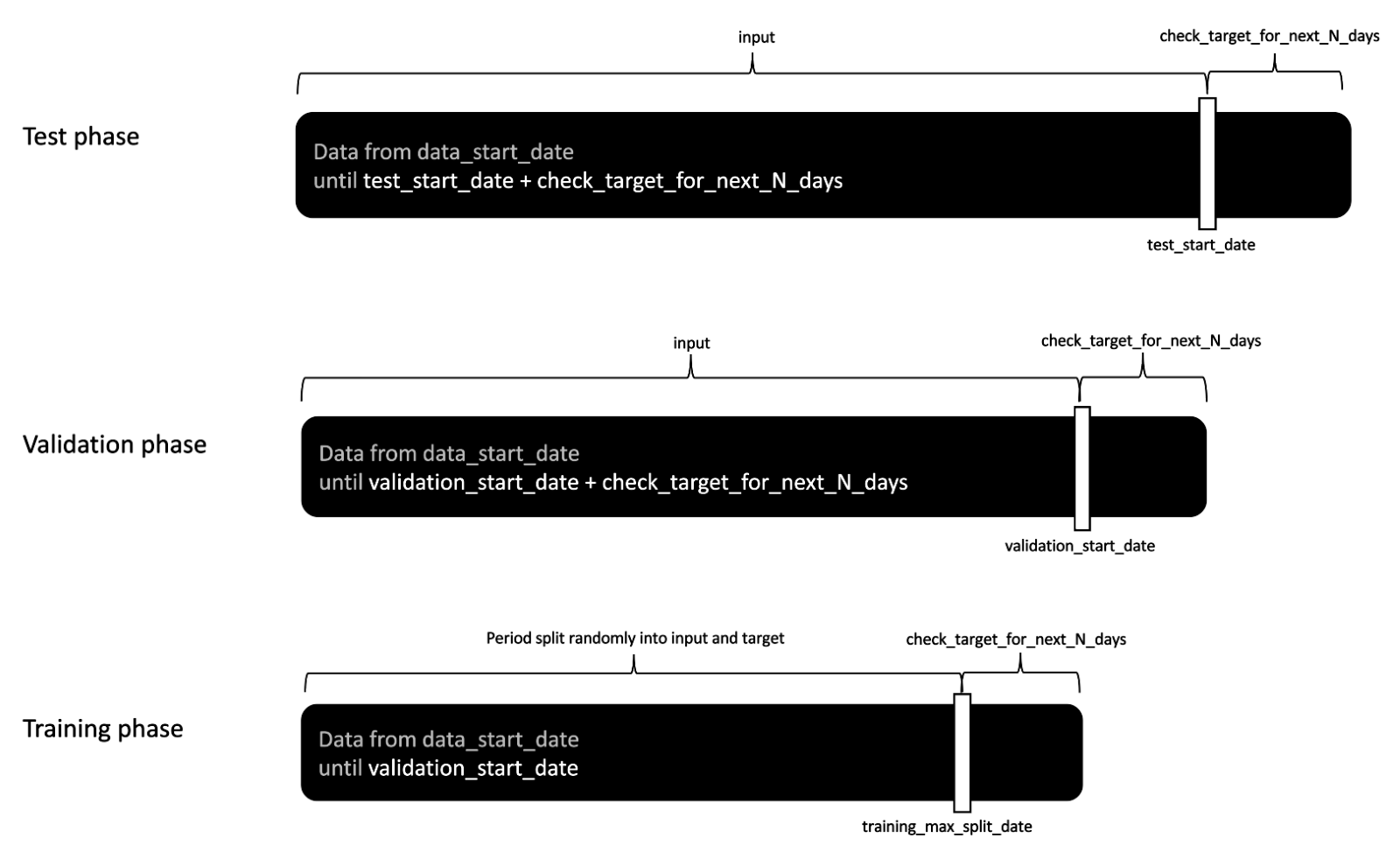
In BaseModel, we introduce the concept of temporal data splits. alternatively of randomly dividing datapoints into 3 distinct sets — train, validation, and test — we divide data in time. First, we establish the dataset starting point, which we will mention to as data start date. From now on, we will only consider data after this date. We can configure it to be the date of the first available data point or, erstwhile working in real-life settings, we may choose to usage a subset of available data, e.g., only data from the last year.
Next, we request to configure the validation start date. Events after this date are not available for training, and we usage them to make targets for validation. Subsequently, we configure the test start date. Data after this date are excluded both from training and validation. However, erstwhile creating model input we always consider data starting from the data start date. This means that in the case of validation, we usage all available data up to the validation start date to make input features and events after the validation start date are what we want to predict. The prediction target, the ground fact for validation is created based on events starting at the validation start date. We check the next n consecutive days for the event we want to predict, e.g., if the product of a given brand or category was bought. This time-window must fit within the period before the test start date to prevent data leakage. To get validation metrics, we compare model results with specified created targets. Similarly, in investigating script all data after the data start date to the test start date are utilized to make an input to the model. The following n days after the test start date are utilized to make targets and measurement model performance.
This method splits data in time alternatively than by users or sessions. We have chosen this approach as we believe it best mimics the real-life scenarios, where models are trained on available historical data and inference is made on events that occurred after training. What is important, in production settings the predictions are made based on the same data origin that was utilized to make the training set. We train a model utilizing the customers' histories that are stored in a data warehouse, and erstwhile a client interacts with the ecosystem, we want to usage available past to supply predictions. erstwhile we measure a model, we should recreate these settings to best represent the context in which the model will be used. erstwhile a different set of users is considered in training and different in validation this creates artificial division devoid of temporal aspects. A simplified, naïve approach of a user-holdout set is besides on our roadmap for fast checks of model stableness during subsequent training sessions.
BaseModel training procedure
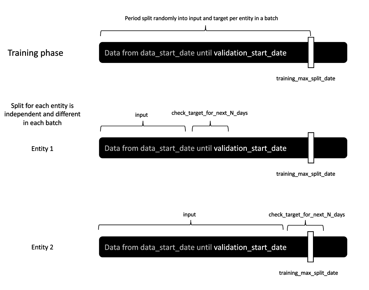
In training, we consider only data after the data start date but before the validation start date. Whereas in validation we usage a fixed date after which we make targets, here, we consider all events that fit into the time window intended for training. Next, we usage event timestamps to choice data divided points, that divide events into 2 chunks — 1 to make input and 1 for targets. What we request to take into consideration is that the latest possible divided point plus the number of days considered to make a mark must fit before the validation start date. It is computed as follows:
training_max_split_date = validation_start_date – 1 – check_target_for_next_N_days
This data divided selection method prevents data leakage — events seen in training will not be utilized to make targets for validation.
When we consider a single user’s history, all events before the divided point are utilized to make input features, and events that occurred during n days after the divided point are utilized to make the model’s target. In standard approaches, a single predefined threshold is set to divide data for training. With our method, multiple divided points can be selected from a single user's history. This way we can augment data by creating multiple data points based on 1 user history.
Recommendations
Although the described data splitting procedures are a general pattern we apply in various tasks from the behavioral modeling domain, in the case of recommendations, we propose a somewhat altered procedure. alternatively of considering the next n days to check the mark we usage the next basket. We observed that this method can improve advice strategy results. However, we supply an option to train recommenders on data beyond 1 basket if needed. In this case, all data from the next n days are utilized and the additional parameter allows you to weigh events with respect to their recency. In the advice task, promoting the model's decisions that are more in line with the most fresh future can boost performance. We can hypothesize that user needs expressed in recommendations depend not only on long-term dependencies but besides on short-term context, which is why predicting the nearest future may improve the quality of recommendations.
Threshold sampling
 Static threshold dates
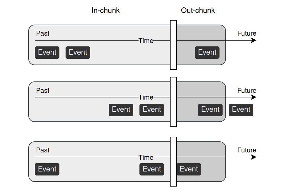
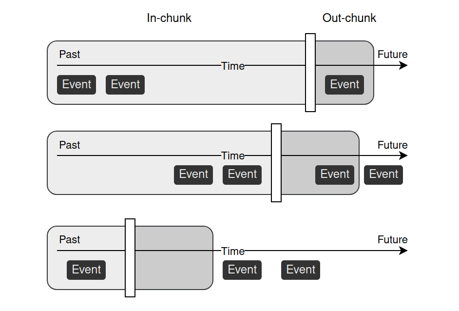
We propose 2 threshold sampling methods: random sampling and valid sampling. In both cases, we randomly choice timestamps from a user’s events, which divides data into 2 chunks: in-chunk for input and out-chunk for target. However, the valid sampling strategy requires at least 1 event in the out-chunk. Whereas random sampling does not gotta fulfill this condition — out-chunks with no events are allowed. This can be a desired behaviour in tasks like churn prediction, where we foretell if a user will make a acquisition in any predefined time window.
 BaseModel random threshold dates
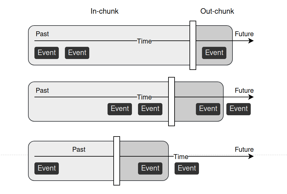 BaseModel
valid threshold dates
BaseModel
valid threshold datesWe supply experiments where we compare these sampling strategies with the standard static approach. In the static approach, 1 threshold is selected, the same for all user, with the anticipation of empty out-chunks. We usage 2 publically available datasets: Kaggle eCommerce dataset and Kaggle H&M dataset. Described sampling strategies are tested in 3 different tasks. In churn prediction, the model is trained to foretell no action in the next 14 days. The propensity model predicts the probability a user will acquisition an item from 1 of the selected brands in the next 14 days. In the advice task, the model is trained to foretell items the user will be curious in over the next 7 days. In the case of churn and propensity prediction, we compare 3 strategies: static, random, and valid. The evaluation metrics for these tasks are the Area Under the Receiver Operating Characteristic Curve (AUROC) and Average Precision (AP). In the case of recommendation, we only consider static and valid sampling as we want the model to always urge something. To measure the advice model we usage Hit Rates at the top 1 and top 10 products returned by the model (HR@1 and HR@10 respectively), as well as Precision at the top 10 products (Prec@10) and mean Average Precision at the top 12 products (mAP@12).
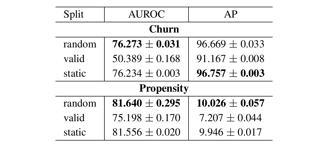 Table 1: Performance of churn and propensity models trained with different time-aware splitting strategies. Results are of the form mean metric value ą standard deviation, computed on 3 independent runs.Table 1: Performance of churn and propensity models trained with different time-aware splitting strategies. Results are of the form mean metric value ą standard deviation, computed on 3 independent runs.
In propensity and churn tasks, the valid sampling method results in worse model performance than another tested methods. Since valid sampling excludes empty out-chunks it results in a distribution that is skewed towards active users. In churn prediction, it explicitly interferes with the task which is to foretell user inactivity. However, propensity task results besides promoted sampling methods that enable an empty time window at a target. This shows that there is information value in users' inactivity and promotes mark created with little purposeful interference with data. On the another hand, the advice task promotes valid sampling over static methods. This suggests that data enrichment with additional samples provides better model results.
 Table 2: Performance of advice models trained with different time-aware splitting strategies, as well as with the static split. Results are of the form mean metric value ą standard deviation, computed on 3 independent runs.
Handcrafted features
These training and evaluation procedures stem from how we realize behavioral modeling problems more generally. The approach to feature engineering plays a decisive function here. Usually, a user is represented by a large vector stored in a feature store. Creating and storing this kind of representation is costly, which makes it hard to make multiple representations for a single user.
Consider a toy example of advice settings. We have information about a user: the unique identifier and (optionally) any attributes like sex or age. We have a past of user interactions with a service, e.g., bought products, page views, add to carts, and so on. We besides may have product attributes, like category, price, size, or brand. The task will be to foretell what the user will buy next. To train any device learning models we request to find a way to represent user past and make input features.
In a naive approach, we may see a list of one-hot encoded products from user history, the average price of bought products, a list of categories the user made a acquisition in, favourite brand. These vectors in fact consist of many handcrafted features which are precomputed and kept in the feature store. Multiple splits will consequence in a radically increased data size that must be stored. Also, aggregated features would request to be re-computed for each fresh data divided to prevent information leakage. For example, if we compute the average price of historical purchases based on 1 data divided and usage the same average price for the earlier split, part of the information from the mark will be available on the input.
Creating features on-the-fly
With BaseModel, we usage our proprietary algorithms to make user representations — Universal Behavioral Representations. These representations are created by combining information from user interactions (events), metadata, and available context into a fixed-size structure. We do not request to store representation for each user. What we store are transform functions learned from data, that supply the mapping between events in user past and fixed-size user representation. We can then choice during training an arbitrary set of events and make user representation on the fly. For details see, Project BaseModel and EMDE Illustrated blog posts.
This method of event data representation is what made our experiments with different data splitting techniques possible, through a fast and lightweight features engineering pipeline. With this flexibility, we were able to augment data by creating multiple data splits from a single user history.