
Pre-processing natural input data is simply a very crucial part of any device learning pipeline, frequently crucial for end model performance. What is more, different fields of ML require different methods to represent applicable information from the input domain in machine-readable format – as numerical vectors. In image processing, we can usage the RGB colour values for each pixel. erstwhile processing texts, things may get more complex, as in most cases we are not curious in how the text looks but what it means. To represent semantic features of a text we usage textual embeddings. They are either trained along with the model or created by learning word co-occurrence in large corpora in a way which helps to encapsulate text meaning. Both operations make multi-dimensional vectors encoding information from images or text.
However, there are quite a few cases where the data is numeric from the beginning. For example, in the financial sector, there are multiple indicators specified as stock prices, marketplace values, revenues; in medical applications, we operate on numerical data representing different body parameters specified as temperature, blood pressure, or oxygen flow; social media is filled with counts of likes, shares, followers or friends. It may seem that we can usage the numeric data straightforwardly as it’s already expressed as numbers. However, to get good results we request to execute any additional steps like data normalization or outlier removal. Usually, to normalize data, we request to compute any statistic across the full dataset – e.g., the mean and standard deviation for a given feature. This can pose any challenges erstwhile analyzing large data streams, where we request to consider time and memory constraints. Also, in many cases, we don’t have all data available up-front. For example, in recommendations, fresh interactions become available as a strategy is being used. We may want to usage them for model fine-tuning, to make it up-to-date with seasonal shifts. However, fresh data may get increasingly inconsistent with previously computed statistics. Also, text or image embeddings are multi-dimensional vectors with 100 dimensions expressing information from a text paragraph or single image. Numerical features describing any phenomena are frequently lower-dimensional, e.g., in medicine.
Fourier encoding of numerical features
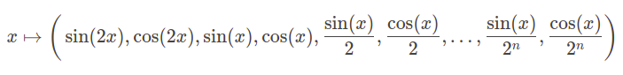
An interesting alternate to normalization for enriching numerical input spaces while obtaining a normalization-like effect & gaining numerical stableness is Fourier feature encoding. The algorithm is alternatively simple, we divide a feature by an expanding scale e.g. \(2^{-1}, 2^{0}, 2^{1}, 2^{2}, 2^{3}, 2^{4}, 2^{5}, 2^{6}\) and we pass each resulting value to the sine and cosine function.
How this transform works and why it’s beneficial is where things get interesting. If we divide a single feature, e.g. representing blood pressure, by values on an expanding 8-level scale and compute sine and cosine functions for each resulting value we get a 16-dimensional vector representing a given value of blood pressure. How is this representation better than a single value? If we look at a sine function, we can see that it can be delicate to tiny changes in input feature value. For example, having these 2 functions we can observe how the same change of x will influence each of them:
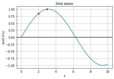
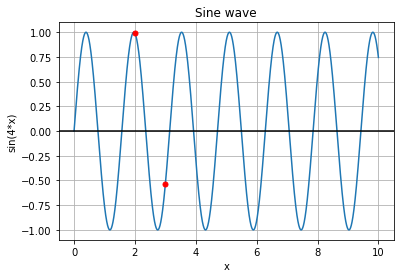
We can see that the lower frequency function will respond to this change in the lower degree and the higher frequency function will capture this change better. By combining functions with different frequencies we represent different levels of sensitivity for changes in input feature value. It may happen that a given function will neglect to capture the change in x:
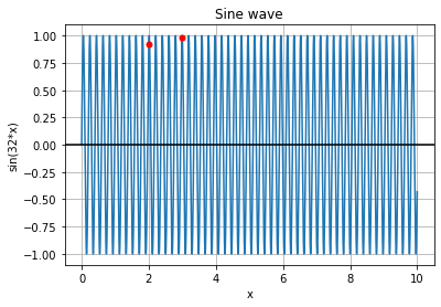
Adding more sines and cosines makes it easier to capture this change.
We map input features from a low-dimensional domain into a higher-dimensional feature space with more complex geometry. This in turn results in a richer gradient and more efficient backpropagation.
Fourier analysis
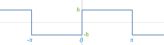
You may inactive wonder why is it called Fourier encoding. This thought has actually a very interesting mathematical background in the field of Fourier analysis. The thought behind it is that any periodic function can be approximated as a sum of sine and cosine waves. Waves that add up to represent a given function come from Fourier analysis. It originated from the reflection (due to Joseph Fourier) that any sufficiently good periodic function can be approximated as a sum of sine and cosine waves. erstwhile we consider square wave:
 (source)
than we take \(sin(x)\):
and \(\frac{\sin(3x)}{3}\):
and add them together:
than we add \(\frac{\sin(5x)}{5}\):
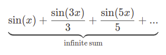
With 17 more sine waves \(\sin(x) + \frac{\sin(3x)}{3} + \frac{\sin(5x)}{5} + ... +\frac{\sin(39)}{39}\) we get:
And 100 sine waves:
Now, we see how we can represent a square wave as a sum of sine waves:
This approximation is called a Fourier (or trigonometric) series of the function. Fourier analysis extends this reflection to a much broader context by introducing alleged Fourier transforms. Trigonometric series is simply a Fourier transform of a periodic function, but Fourier transforms are defined for much more general classes of functions and signals. Regardless of method details, the intuition is that the Fourier transform is utilized to decompose a signal or function onto frequencies that constitute it.
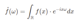
For the signals in the time domain, we can describe Fourier transform in the following way. Let \(f:\mathbb{R}\rightarrow \mathbb{C}\) be a complex time signal and \(\omega\ \in \mathbb{R}\) be a frequency. Then Fourier transform of \(\hat{f}\) of \(f\) evaluated at \(\omega\) is given by the formula
Provided example was related to time signals (for \(\mathbb{R}\)) but Fourier analysis can be applied much broader. It is commonly utilized in many fields of discipline specified as engineering, physics, and chemistry. A popular application of discrete Fourier transform is for image processing, filtering, reconstruction, or compression.
Spectral bias of multilayer perceptron
Using Fourier analysis Rahman et al. investigated spectral features (metrics in frequency domain) of multilayer perceptron (MLP) with ReLU activation function. They observed that low-frequencies are learned faster than high-frequencies and called this phenomenon spectral bias. It means that global patterns are easier and quicker to learn and approximate than local fluctuations. For example, if we have a picture, the network will tend to represent it in a blurrier way, paying attention to the general pattern and omitting sharper elements or object edges. Sometimes this can be viewed as the desired behaviour – a form of implicit regularization. However, in another cases, we may want the model to pay attention to fine-grained detail. Rahman et al. besides observed that enriching input data with high-frequency components facilitates model training. Going back to a blurry image example, we can inspect the impact of described input modifications erstwhile we train a MLP network to memorize an image. In this setting, the network learns to foretell RGB colour values for each pixel based on its coordinates. Regular MLPs conflict with learning specified functions, which is clearly visible in the blurry image below. However, erstwhile we usage Fourier feature mapping proposed by Tancik et al., we can see that the learned image is much sharper. Enriching input feature space geometry allowed the model to learn high-frequency components much faster:
Transformer positional encoding
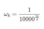
Another good example of this thought is positional encoding in Transformer architecture. Transformer architecture, based on the self-attention mechanism, is primarily utilized in language processing where word sequences service as model input. Contrary to Recurrent Neural Networks, which process input tokens 1 by one, pure Transformers are permutation invariant and do not have information about the positions of input tokens. To add this information, model input is enriched with positional embeddings which encode tokens's position in a sequence. The position is encoded with the following formula, where \(t\) represents a token position in the input sequence, \(p_t\) is a position encoding vector, \(d\) is simply a vector dimension and \(f\) is simply a function producing \(p_t\) vector:
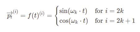
where
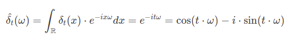
What‘s the intuition behind this formula? We can interpret a word with position \(t\) in a series as an impulse in the time domain – Dirac delta \(\delta_t\). This way we know that its Fourier transform will be complex exponential, since according to the expression introduced in Fourier analysis paragraph:
Now, if we look at the Fourier transform and positional encoding function, we can see the similarity. In fact, sampling provided Fourier transform function at points \(\omega_k\) for \(k=0,1,…,\frac{d}{2}\) and inserting these sampled values into a single vector produces positional encoding. We can interpret it as a representation of word position in frequency domain.
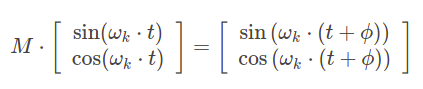
An interesting hypothesis from the paper introducing Transformer, Attention is all you need, is that positional encoding allows the model to easy learn comparative positioning. The claim stems from the fact that for any fixed offset \(\phi\) there is simply a linear transformation from \(p_t\) to \(p_{t+\phi}\) that holds for any position \(t\). For each sine and cosine pair with a given frequency we can find 2x2 transformation matrix \(M\) such that:
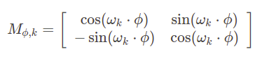
and the matrix for a given \(\phi\) can be found independently from the position t with provided expression (see a proof):
It was hypothesized that models would be able to easy utilize this comparative positioning strategy to facilitate extrapolation to longer sequences.
However, more recently, Press et al. showed that Transformer positional encodings can only extrapolate input sizes to a limited degree without affecting model performance. erstwhile more than 50 additional tokens are added during inference than in training, the performance begins to drop significantly. They proposed a fresh architecture – ALIBI, which adds a constant bias to attention scores alternatively of explicitly modeling positions as vectors. The bias is multiplied by head-specific scalar m:
This solution can extrapolate to much longer sequences without a crucial drop in performance. If you want to know the details of this solution see paper describing ALIBI architecture.
The Transformer extrapolation use-case is rather special, and while positional encodings are slow becoming obsolete for language models, Fourier feature encoding has much wider uses.
Our usage cases
At Synerise we usage it with numerical features to make higher dimensional and more complex representations while sidestepping the necessity for explicit normalization.
We were able to validate the general applicability of Fourier encoding for numeric variables in the RecSys Twitter challenge, where we presented the second-best solution. The task was to foretell if a given user will respond to a Tweet. Fourier encoding was utilized to encode all numerical features specified as the number of followers, hashtags, time since account creation, etc. We besides utilized Fourier feature encoding in KDD Cup 2021, where we obtained 3rd place. The nonsubjective was to foretell the subject area of papers in a large-scale academic graph. We encoded features like the number of cited papers, number of authors, or publication year. We besides utilize this method in Synerise Monad - a platform for automatic creation of behavioral profiles from natural data.
Experimental results
To show the impact of Fourier feature encoding alone we prepared a simple experimental setting. We utilized Pima Indians Diabetes dataset, where the nonsubjective is to foretell a diabetes diagnosis based on provided diagnostic measurements:
import pandas as pd csv_file='diabetes.csv' df = pd.read_csv(csv_file) df.head(10)We trained a simple MLP with 1 hidden layer. To reasonably compare the results, we utilized hidden size 100 for the model with explicit normalization and hidden size 6 for the model utilizing Fourier feature encoding. This way we kept the full number of learnable parameters constant, despite different input sizes. For the explicit normalization, we utilized sklearn’s StandardScaler.
import numpy as np from sklearn.neural_network import MLPClassifier from sklearn.preprocessing import StandardScaler from sklearn.model_selection import cross_validate X = df.iloc[:,:-1].values y = df.iloc[:,-1].values scaler = StandardScaler() X_scaled = scaler.fit_transform(X) mlp = MLPClassifier(hidden_layer_sizes=(100,), random_state=8, alpha=1, max_iter=400, learning_rate_init=0.005, verbose=True) res = cross_validate(mlp, X_scaled, y, cv=5)For Fourier encoding, we utilized an 8-level scale with successive powers of three. Here we supply a code example for Fourier encoding of feature column:
def multiscale(x, scales): return np.hstack([x.reshape(-1, 1)/pow(3., i) for i in scales]) def encode_scalar_column(x, scales=[-1, 0, 1, 2, 3, 4, 5, 6]): return np.hstack([np.sin(multiscale(x, scales)), np.cos(multiscale(x, scales))]) X = np.apply_along_axis(encode_scalar_column, axis=0, arr=X) X = X.reshape((-1, X.shape[-2] * X.shape[-1]), order="F") mlp = MLPClassifier(hidden_layer_sizes=(6,), random_state=8, alpha=1, max_iter=400, verbose=True) res = cross_validate(mlp, X, y, cv=5)We trained the models with 5-fold cross-validation and measured model performance in terms of accuracy. Averaged results from 5 train/test splits:
MLP no feature normalization: 0.66MLP + StandardScaler: 0.78
MLP + Fourier feature encoding: 0.78
We can see that Fourier feature encoding enhanced model performance importantly in comparison to unnormalized data and obtained the same results as standard normalization. This example shows that Fourier feature encoding can increase the expressive power of numerical features and enable easier learning for neural networks. At the same time, it side-step the request for dataset statistic computation, which makes it a good method to usage with large data streams and for continuous training, where models are periodically updated with fresh data.